Output files
epic can produce many output files. Here we explain what they contain.
-o/–outfile
The main output is the file of regions with an FDR score lower than the cutoff (0.05 by default).
# epic -cpu 25 -t examples/test.bed -c examples/control.bed -o enriched_regions.csv
Chromosome Start End ChIP Input Score Log2FC P FDR
chr1 23568400 23568599 2 0 13.54464274405703 11.30748585550573 8.184731894908448e-11 6.319374393278151e-10
chr1 26401200 26401399 2 0 13.54464274405703 11.30748585550573 8.184731894908448e-11 6.319374393278151e-10
chr1 33054800 33055399 2 0 14.288252844518933 9.722523354784574 2.207263610333191e-09 3.85690272963484e-09
chr1 33365200 33365399 2 0 13.54464274405703 11.30748585550573 8.184731894908448e-11 6.319374393278151e-10
chr1 39422200 39422799 2 0 14.288252844518933 9.722523354784574 2.207263610333191e-09 3.85690272963484e-09
chr1 51473600 51474399 2 0 14.288252844518933 9.30748585550573 5.228937118152232e-09 6.861688234097e-09
chr1 58785200 58786199 2 0 14.288252844518933 8.985557760618368 1.0206726421638307e-08 1.1002055753194539e-08
chr1 59430000 59430199 2 0 13.54464274405703 11.30748585550573 8.184731894908448e-11 6.319374393278151e-10
The first two lines are special and do not contain any data:
- The first line contains the command invoked
- The second line contains the column names
The column names are:
- Chromosome, Start, End
This is the location of the region.
- ChIP, Input
These two columns contain the number of ChIP-reads and Input-reads within the region.
- Score
(Mostly uninteresting to end users). This is the region Poisson score.
- Fold_change
The log2_fold change is the number of ChIP reads divided by the number of Input reads in the region (where a pseudocount is computed for regions with no input-reads.)
- P
This is the p-value, based on the Poisson-distribution.
- FDR
FDR is the p-value adjusted for multiple testing with Benjamini-Hochberg.
-b/–bed (optional)
This is a bed file of the regions. This file is intended for downstream analyses with tools like bedtools or for display in the UCSC genome browser. (As opposed to the –output file which contains more statistical info and the read counts for a region and is not usable as-is by most tools.)
The three first columns are the region, the fourth is the FDR score (same as in the –outfile), and the fifth contains the log2 fold change * 100 capped at 1000. The sixth contains the strand, but ChIP-Seq data is not stranded.
chr1        23568400        23568599        6.319374393278151e-10   1000.0  .
chr1        26401200        26401399        6.319374393278151e-10   1000.0  .
chr1        33054800        33055399        3.85690272963484e-09    1000.0  .
chr1        33365200        33365399        6.319374393278151e-10   1000.0  .
chr1        39422200        39422799        3.85690272963484e-09    1000.0  .
chr1        51473600        51474399        6.861688234097e-09      1000.0  .
chr1        58785200        58786199        1.1002055753194539e-08  1000.0  .
chr1        59430000        59430199        6.319374393278151e-10   1000.0  .
chr1        65065600        65066199        3.85690272963484e-09    1000.0  .
chr1        91625400        91625799        1.8569048582126885e-09  1000.0  .
-sm/–store-matrix
This option gives a matrix of counts for each genomic bin (tile/window) for all the bed/bedpes given to epic. It is intended for downstream statistical analyses. It is gzipped since it can be enormously big.
Chromosome, Bin
The two first columns give the location of the bin (window).
Enriched
This column tells whether the bin was part of an enriched region (according to the FDR cutoff given to epic). 0 means no and 1 means yes.
chip1.bed, input1.bed, …, chipn.bed, inputn.bed
The next columns are the files used in the epic analysis and contain the read-count for each bin. In the example below the files used are examples/test.bed and examples/control.bed so this is what the columns are called too.
epic -t examples/test.bed -c examples/control.bed -sm matrix.gz > /dev/null
zcat matrix.gz  | head # gzcat on some mac OSes
# Chromosome Bin Enriched examples/test.bed examples/control.bed
# chr1 887600 0 0 1
# chr1 994600 0 0 1
# chr1 1041000 0 0 1
# chr1 1325200 0 1 0
# chr1 1541600 0 1 0
# chr1 1599000 0 1 0
# chr1 1770200 0 0 1
# chr1 1820200 0 1 0
# chr1 1995000 0 0 1
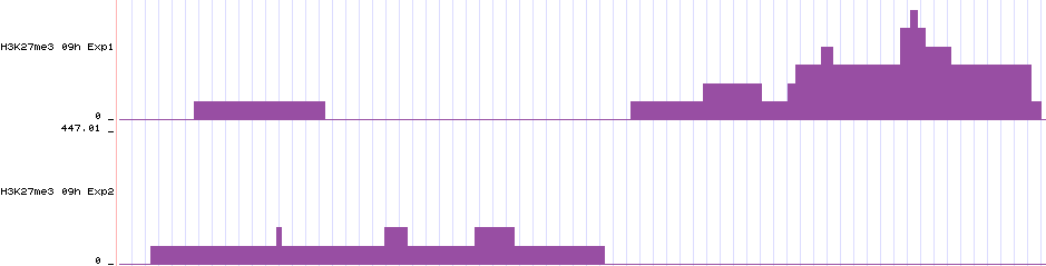
-bw/–bigwig (optional)
This flag takes a folder to store bigwigs in. One bigwig file is created per bed/bedpe file given for epic to analyze. The scores are RPKM-normalized.
epic -bw bigwigs/ -t examples/test.bed -c examples/control.bed \
            -o examples/expected_results_log2fc.csv
ls bigwigs/
# control.bw test.bw
These bigwigs show how epic saw the data. So the data will look like a histogram where the bars are bins and the counts within a bin gives the height of the bar. The results are RPKM-normalized. Here are two bigwigs displayed in an arbitrary genomic region in the UCSC genome browser:
-i2bw/–individual-log2fc-bigwigs
This flag takes a folder to store bigwigs in. One bigwig file is created per ChIP bed/bedpe file given for epic to analyze. The scores are RPKM-normalized and divided by the mean of the summed input RPKM. A pseudocount of one is given to bins with no input. I is the number of Input-files in the equation below:
-cbw/–chip-bigwig
The ChIP-bigwig creates a common bigwig for all the ChIP-Seq files. First the RPKM is computed for each bed/bedpe file, then these are added together and the –chip-bigwig is produced.
The value in each bin is (where C is the number of ChIP-files):
-ibw/–input-bigwig
The Input-bigwig creates a common bigwig for all the input files. First the RPKM is computed for each bed/bedpe file, then these are added together and the –input-bigwig is produced.
The value in each bin is (where I is the number of Input-files):
-2bw/–log2fc-bigwig
Sums of the RPKM-scores for each library is computed like described in -cbw and -ibw. Then a pseudocount of one is added to each bin with a count of zero in the input. Finally the summed ChIP and Input vectors are divided and then the log2 is computed.
-l/–log
Write all the logging messages to a file (in addition to stderr).